Description
Calculate and plot r and Cohen’s d effect size and its confidence intervals.
Usage
effsize_plot(x, g, method = 'r', paired = F,
             color = 'black', size = 2,
             width = .05,
             line.col = 'grey', lwd = 1, lty = 2,
             ggtheme = theme_minimal(),
             par_r = list(conf = .95, type = 'perc', R = 1000),
             par_d = list(pooled = T, hedges.correction = F, conf.level = .95),
             plot = T, show = F)
Arguments
x, g: dataframe and vector with numerical and factor variables, respectively.
method: specify what effect size to compute: Wilcoxon r ('r') or Cohen’s d ('d').
paired: logical. Whether samples are paired (default = F).
color, size: character or hexa specifying the errorbar and point colours, and size of points, respectively.
width: width of errorbar brackets.
line.col, lwd, lty: colour, width and type of the zero-crossing line, respectively.
ggtheme: a ggplot2 theme function.
par_r: list of parameters to be passed to WilcoxonR or WilcoxonPairedR functions. Specify as list(conf, type, R), where conf is the level of confidence interval, type is the type of bootstrap estimation for confidence interval (‘norm’ for …, ‘basic’ for …, ‘perc’ for …, ‘bca’ for …) and R is the number of bootstrap resampling.
par_d: list of parameters to be passed to cohen.d function. Specify as list(pooled, hedges.correction, conf.level), where pooled is a logical indicating whether should be used the pooled standard deviation (TRUE, default) or the whole sample standard deviation (FALSE), hedges.correction is a logical indicating if Hedges correction should be applied (TRUE) or not (FALSE, default) and conf.level is the level of the confidence inteval.
plot: logical indicating whether to plot (TRUE, default) or not (FALSE)
show: logical indicating whether to print the estimate, p-value, effect size and its confidence intervals (TRUE) or not (FALSE, default).
Details
The packages rcompanion1 and effsize2 are required to calculate r and d/g effect size, respectively.
For more details about how each effect size is calculated, read the documentation of rcompanion and effsize.
Value
A list comprised of:
es_plot the plot output.
metrics a data.frame with variable names, statistic (t or W/V), p-value, effect size (r or d/g) and lower and upper limits of confidence interval.
Examples
Generating dataset
x <- factor(rep(c('A','B'), each = 50))

y1 <- abs(rnorm(100, mean = 8.4, sd = 2)) %>% round(.,0)
y1[51:100] <- abs(rnorm(50, 10, 4)) %>% round(.,0)

y2 <- abs(rnorm(100, 25, 5)) %>% round(.,0)
y2[51:100] <- abs(rnorm(50, 23.3, 4)) %>% round(.,0)

y3 <- abs(rnorm(100, 8.5, 4)) %>% round(.,0)
y3[51:100] <- abs(rnorm(50, 11.2, 5.5)) %>% round(.,0)

df <- data.frame(x,y1,y2,y3)
Loading the function
source('https://github.com/geovanjr/stats/raw/master/effsize_plot.R')
Calculating r effect size
effsize_plot(df[,2:4], df[,1], method = 'r', paired = F, plot = T, show = T,
             color = 'forestgreen',
             par_r = list(R = 500))
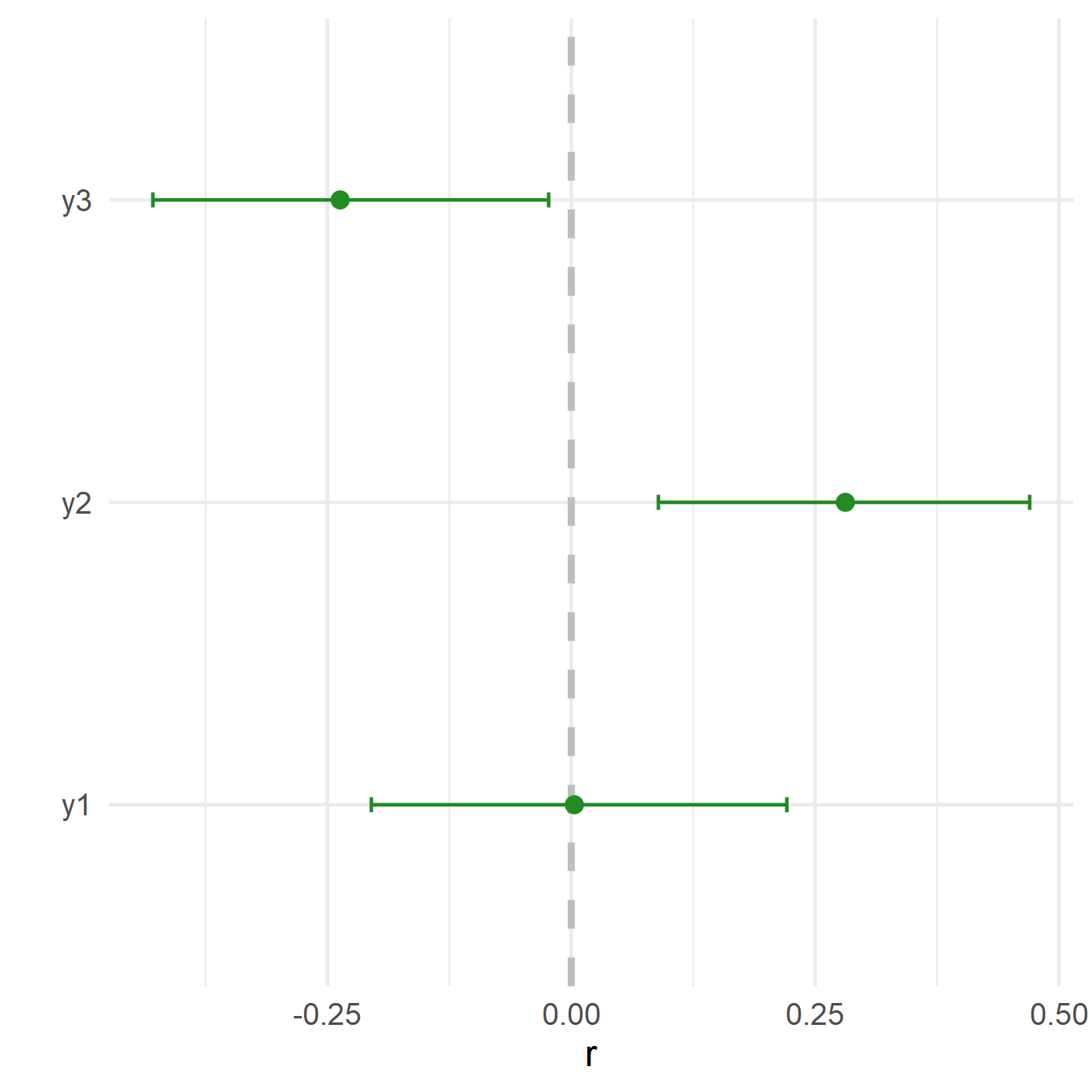
##   variable      W      p      r   lower   upper
## 1       y1 1176.5 0.6122 -0.051 -0.2620  0.1660
## 2       y2 1470.5 0.1283  0.152 -0.0779  0.3720
## 3       y3  911.0 0.0192 -0.234 -0.4210 -0.0411
Calculating d effect size
effsize_plot(df[,2:4], df[,1], method = 'd', paired = F, plot = T, show = T,
             color = 'forestgreen', size = 3, lty = 3, ggtheme = theme_light())
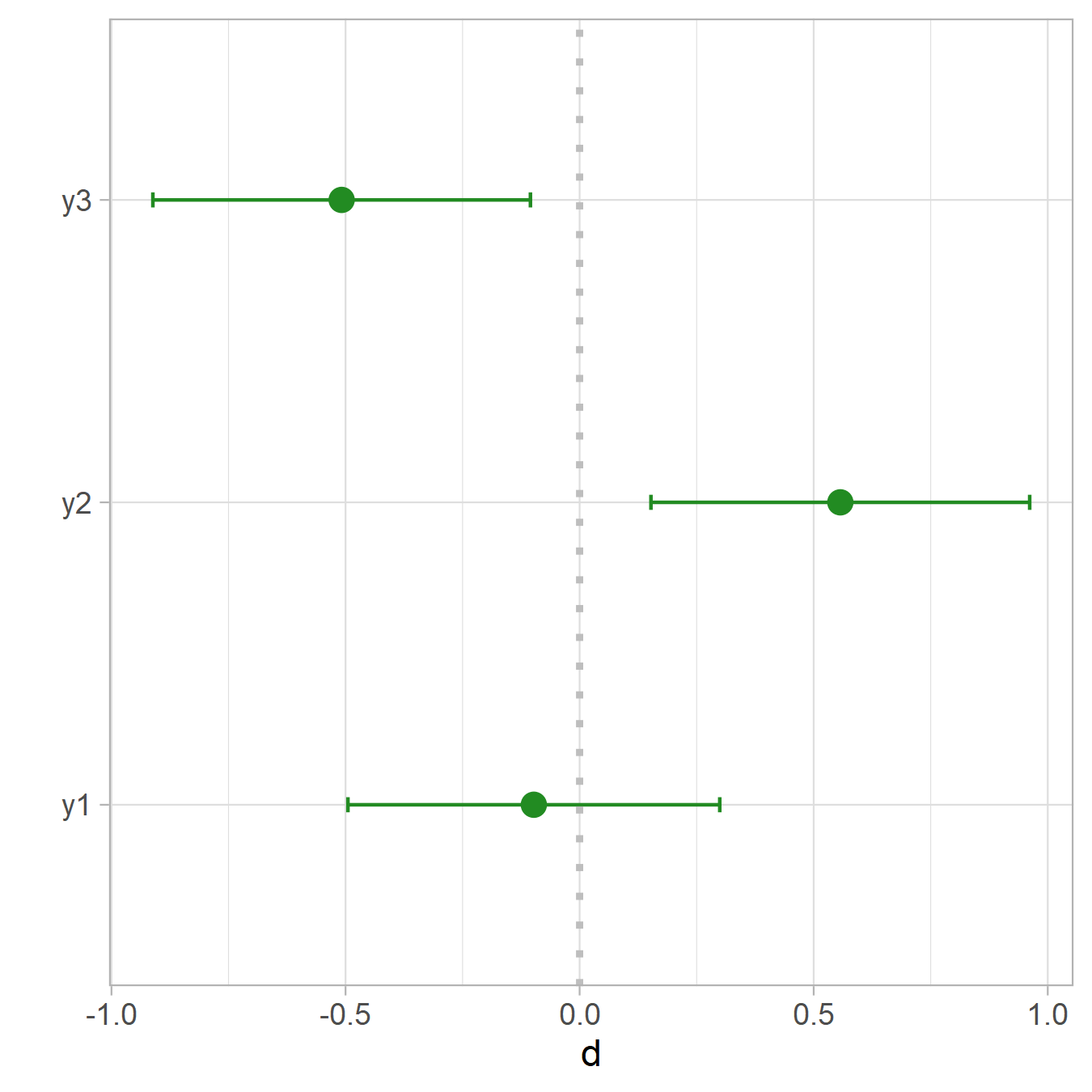
##   variable          t      p          d       lower       upper
## 1       y1 -0.9761759 0.3325 -0.1952352 -0.59307307  0.20260270
## 2       y2  1.8059423 0.0743  0.3611885 -0.03892805  0.76130495
## 3       y3 -2.4013729 0.0186 -0.4802746 -0.88284923 -0.07769995
Calculating g effect size
effsize_plot(df[,2:4], df[,1], method = 'd', paired = F, plot = T, show = T,
             color = 'forestgreen', size = 3, lty = 3,
             par_d = list(hedges.correction = TRUE))
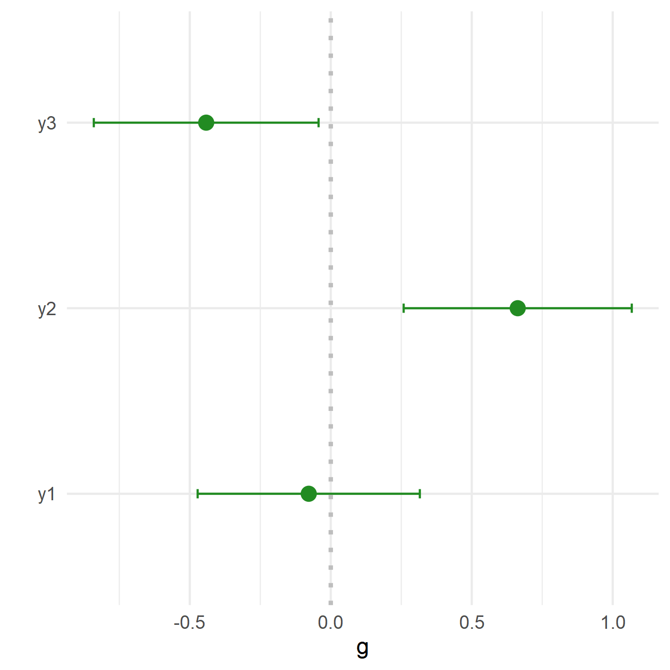
##   variable          t      p          g       lower       upper
## 1       y1 -0.9761759 0.3325 -0.1488374 -0.54323056 0.245555825
## 2       y2  1.8059423 0.0743  0.4273615  0.02904288 0.825680139
## 3       y3 -2.4013729 0.0186 -0.3932010 -0.79083675 0.004434836
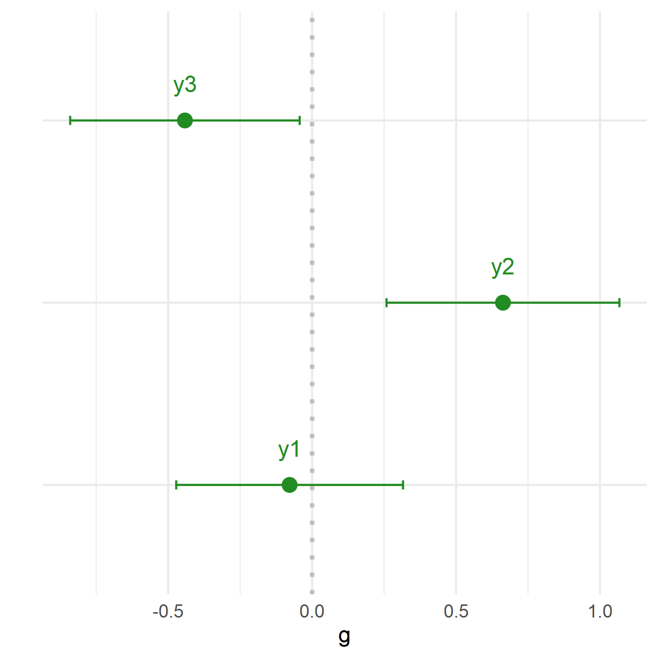
Changing es_plot aesthetics
es <- effsize_plot(df[,2:4], df[,1], method = 'd', paired = F, plot = F, show = F,
             color = 'forestgreen', size = 3, lty = 3,
             par_d = list(hedges.correction = TRUE))

es$es_plot +
  theme(axis.text.y = element_blank()) +
  annotate('text', 1+.2, es$metrics[1,4],
           label = paste0(es$metrics[1,1]),
           size = 4, color = 'forestgreen') +
  annotate('text', 2+.2, es$metrics[2,4],
           label = paste0(es$metrics[2,1]),
           size = 4, color = 'forestgreen') +
  annotate('text', 3+.2, es$metrics[3,4],
           label = paste0(es$metrics[3,1]),
           size = 4, color = 'forestgreen')
Getting metrics
es$metrics
| variable | t | p | g | lower | upper |
|---|---|---|---|---|---|
| y1 | -0.9761759 | 0.3325 | -0.1488374 | -0.5432306 | 0.2455558 |
| y2 | 1.8059423 | 0.0743 | 0.4273615 | 0.0290429 | 0.8256801 |
| y3 | -2.4013729 | 0.0186 | -0.3932010 | -0.7908367 | 0.0044348 |
References
- Salvatore Mangiafico (2020). rcompanion: Functions to Support Extension Education Program Evaluation. R package version 2.3.25. https://CRAN.R-project.org/package=rcompanion
- Torchiano M (2020). effsize: Efficient Effect Size Computation. doi: 10.5281/zenodo.1480624 (URL: https://doi.org/10.5281/zenodo.1480624), R package version 0.8.0, <URL: https://CRAN.R-project.org/package=effsize>.